Download a Financial Analysis Model designed by Wael Abed, Financial Modeling Expert.
Introduction: Why Excel Remains the King of Financial Analysis
In the fast-paced world of modern finance, the ability to transform raw, chaotic data into clear, actionable intelligence is what separates industry leaders from the rest. While new BI tools emerge constantly, Microsoft Excel remains the undisputed cornerstone of this analytical transformation. A deep, practical mastery of Financial Analysis in Excel is not just a resume bullet point; it is a fundamental language spoken in boardrooms, trading floors, and finance departments globally. Whether you are forecasting revenue, valuing an investment, optimizing cash flow, or simply tracking departmental budgets, Excel provides an unrivalled toolkit. This definitive guide is designed to be your comprehensive manual, taking you from a competent user to a virtuoso of Financial Analysis in Excel. We will delve into essential functions, advanced modeling, powerful data visualization, and professional best practices, all illustrated with practical examples you can apply immediately.
For a deep dive into all our resources on this topic, explore our complete archive in the Financial Analysis category.
Chapter 1: Excel Fundamentals for Effective Financial Analysis
Before executing complex maneuvers, every expert must perfect their stance. A robust analytical process in Excel begins with impeccable data structure and hygiene.
1.1. Structuring Financial Data for Excel Analysis
The single biggest mistake in Excel is poor source data structure. For seamless analysis, especially with PivotTables, follow these rules:
- Use Excel Tables: Always convert your data range into a formal Excel Table (
Ctrl + T). This ensures automatic formula expansion, easy filtering, and dynamic ranges that are crucial for scalable Financial Analysis in Excel. - One Header per Column: Each column should represent a single variable (e.g.,
Date,Product_ID,Region,Revenue,Cost). - One Row per Record: Each row should represent a unique transaction or data point.
- No Merged Cells: Merged cells are the arch-nemesis of formulas, sorting, and PivotTables. Use « Center Across Selection » for formatting instead.
1.2. Excel Shortcuts for Financial Analysis Efficiency
Efficiency is currency for a financial analyst.
| Shortcut | Action |
|---|---|
Ctrl + [Arrow Key] | Navigate to the edge of the data region |
Ctrl + Shift + L | Toggle AutoFilters on/off |
Alt + = | AutoSum selected cells |
Ctrl + Page Up/Down | Navigate between worksheets |
F2 | Edit the active cell |
Ctrl + ~ | Toggle Formula View |
Chapter 2: Essential Excel Formulas for Financial Analysis
Mastering formulas is the first step to unlocking Excel’s power. Here is your essential toolkit.
2.1. Key Excel Functions for Financial Analysis
- SUMIFS: The workhorse for conditional aggregation.
=SUMIFS(Sum_Range, Criteria_Range1, Criteria1, ...)- Example:
=SUMIFS(Sales_Amount, Region, "North", Product, "Widget A")
- XLOOKUP: The modern, powerful successor to VLOOKUP. It looks up a value in a range and returns a corresponding value from another range.
=XLOOKUP(Lookup_Value, Lookup_Array, Return_Array, [If_Not_Found])- Example:
=XLOOKUP(A2, Product_List, Price_List, "Not Found")
- INDEX/MATCH: A flexible and robust alternative for complex lookups. While XLOOKUP is often better, this combo is still vital for legacy sheets and specific scenarios.
=INDEX(Return_Column, MATCH(Lookup_Value, Lookup_Column, 0))
- IFS / SWITCH: For clean, multi-condition logic.
=IFS(A2>100, "High", A2>50, "Medium", TRUE, "Low")
- IFERROR / IFNA: To create clean, professional models by handling errors gracefully.
=IFERROR(Your_Formula, "Value if Error")
- EDATE / EOMONTH: Critical for date-based calculations in financial modeling (e.g., calculating maturity dates).
=EDATE(Start_Date, 6)returns the date 6 months after the start date.
- SUMPRODUCT: A versatile function for weighted averages, conditional sums with multiple criteria, and array operations before dynamic arrays.
=SUMPRODUCT((Region="North")*(Product="Widget A")*Sales)
- UNIQUE & FILTER: New Dynamic Array functions that revolutionize data extraction and listing.
=UNIQUE(A:A)spills a list of unique values from column A.=FILTER(A:B, A:A="North")spills all rows where the region is « North ».
- SEQUENCE: Generates a list of sequential numbers. Incredible for building timelines and schedules.
=SEQUENCE(12)generates a vertical array from 1 to 12.
- LET: Allows you to assign names to calculation results within a formula. This improves readability and performance for complex formulas.
=LET(x, A1*10, y, B1*0.5, x+y)
XLOOKUP: The modern, powerful successor to VLOOKUP. For those still using the legacy function, our comprehensive VLOOKUP Formula Guide with Examples covers all scenarios and limitations.
2.2. Practical Financial Analysis Examples in Excel
Let’s use these functions to create a dynamic summary table from a raw transaction log.
Raw Data (Table named tblSales):
| Date | Region | Product | Salesperson | Revenue |
|---|---|---|---|---|
| 01/01/2025 | North | Widget A | Alice | $1,000 |
| 01/01/2025 | South | Widget B | Bob | $1,500 |
| … | … | … | … | … |
Summary Report Formula:
excel
=LET(
    Regions, UNIQUE(tblSales[Region]),
    Products, UNIQUE(tblSales[Product]),
    HSTACK(Regions, SUMIFS(tblSales[Revenue], tblSales[Region], Regions))
)
This single formula creates a unique list of regions and their total revenue next to it.
Chapter 3: Financial Modeling and Investment Analysis in Excel
Excel has a dedicated suite of functions for core financial calculations. To get the most out of these, it’s best to understand the underlying theory. You can learn more about the theory behind these calculations on Investopedia’s Financial Modeling guide.
3.1. Financial Investment Analysis Using Excel Functions
- NPV (Net Present Value): Calculates the present value of a series of future cash flows. A positive NPV indicates a profitable project.
=NPV(Rate, Cashflow1, Cashflow2, ...)- Pro Tip: Your initial investment (usually a negative cash outflow at time 0) is often not included in the NPV function’s arguments. It’s added separately:
=NPV(Rate, CF1:CFn) + CF0. For more precise timing, use=XNPV(Rate, Cashflows, Dates).
- IRR (Internal Rate of Return): The discount rate that makes the NPV of all cash flows equal to zero. It’s the project’s expected compound annual rate of return.
=IRR(Cashflow_Range, [Guess])- Warning: IRR can be misleading for non-conventional cash flows and should always be analyzed alongside NPV.
3.2. Excel Calculations for Financial Planning
- PMT (Payment): Calculates the periodic payment for a loan.
=PMT(Rate, Nper, Pv, [Fv], [Type])- Example:
=PMT(5%/12, 5*12, 200000)calculates the monthly payment for a $200,000 loan at 5% annual interest over 5 years.
- SLN & DB (Depreciation):
- SLN: Calculates straight-line depreciation.
=SLN(Cost, Salvage, Life) - DB: Calculates declining balance depreciation.
=DB(Cost, Salvage, Life, Period, [Month])
- SLN: Calculates straight-line depreciation.
PMT (Payment): Calculates the periodic payment for a loan. =PMT(Rate, Nper, Pv, [Fv], [Type]). For a deep dive with practical examples, see our dedicated tutorial on the Excel PMT Function
3.3. Practical Exercise: Project Comparison
Build a model to compare two potential projects.
Project A & B Cash Flows:
| Period | Project A | Project B |
|---|---|---|
| 0 | -$150,000 | -$200,000 |
| 1 | $45,000 | $30,000 |
| 2 | $50,000 | $50,000 |
| 3 | $55,000 | $70,000 |
| 4 | $40,000 | $90,000 |
| 5 | $35,000 | $50,000 |
Analysis Formulas:
| Metric | Formula (for Project A) | Result A | Result B |
|---|---|---|---|
| NPV (8% Rate) | =NPV(8%, B3:B7) + B2 | $33,237 | $32,458 |
| IRR | =IRR(B2:B7) | 15.2% | 14.8% |
Based on this analysis, Project A has a slightly higher NPV and IRR, making it the more attractive investment.
Chapter 4: Data Analysis Techniques for Financial Professionals
If you only master one feature in Excel for Financial Analysis in Excel, it must be the PivotTable. It is the ultimate tool for data summarization and exploration.
4.1. Financial Data Analysis with PivotTables
- Click anywhere inside your Excel Table.
- Go to
Insert > PivotTable. - Choose to place it in a new worksheet.
- Use the drag-and-drop PivotTable Fields pane:
- Filters: For global report filters (e.g.,
Year). - Rows: Your categories (e.g.,
Region,Product). - Columns: For sub-categorization (e.g.,
Quarter). - Values: The data to summarize (e.g.,
Sum of Revenue,Average of Margin).
- Filters: For global report filters (e.g.,
4.2. Advanced PivotTable Techniques
- Calculated Fields & Items: Create your own formulas within the PivotTable. For example, add a
"Margin %"field as=Margin / Revenue. - Show Values As: Right-click a value >
Show Values As. This allows you to display data as% of Grand Total,% of Parent Row Total, orDifference Fromprevious period—incredibly powerful for variance analysis. - Grouping: Group dates by months, quarters, and years automatically. Group numbers into bins.
4.3. The Data Model & Power Pivot: A Game Changer
For analyzing millions of rows and creating complex relationships between multiple tables, you must use the Data Model with Power Pivot.
- Create Relationships: Link your
Salestable to aProductstable and aCalendartable on common keys (likeProduct_IDandDate). - Use DAX Formulas: Data Analysis Expressions (DAX) is a formula language for creating custom calculations.
Total Sales = SUM(Sales[Revenue])Sales YTD = TOTALYTD([Total Sales], 'Calendar'[Date])Sales YoY Growth = ([Total Sales] - CALCULATE([Total Sales], SAMEPERIODLASTYEAR('Calendar'[Date]))) / CALCULATE([Total Sales], SAMEPERIODLASTYEAR('Calendar'[Date]))
Building a proper star schema with the Data Model is the foundation of professional Financial Analysis in Excel.
Chapter 5: Building Professional Financial Models in Excel
A financial model is a mathematical representation of a company’s or project’s financial performance. It is the pinnacle of applied Financial Analysis in Excel.
5.1. Building Integrated Financial Statements in Excel
A robust model connects three core statements.
- Assumptions Sheet: All driver inputs are here (growth rates, margins, working capital days, tax rate).
- Income Statement: Built from revenue assumptions down to Net Income.
- Balance Sheet: Assets, Liabilities, and Equity must balance (
Assets = Liabilities + Equity). This is your primary check for model integrity. - Cash Flow Statement: Reconciles Net Income to the change in Cash, using the indirect method. It should link directly to the Balance Sheet.
5.2. Key Modeling Concepts
- Circular References & the Iterative Calculation Switch: A circularity occurs when a formula refers to its own cell, either directly or indirectly. While often an error, they are sometimes necessary (e.g., calculating interest on cash). Handle with care and use
File > Options > Formulas > Enable iterative calculationif needed. - The Cash Flow Waterfall: The most critical link. Your model must correctly calculate:
- Operating Cash Flow: Starts with Net Income, adds back non-cash items, and adjusts for changes in Working Capital.
- Investing & Financing Cash Flows: From capital expenditures and debt issuances/repayments.
- Ending Cash: Must equal
Beginning Cash + Net Change in Cashfrom the Cash Flow Statement.
5.3. Scenario Analysis with Data Tables
What-if analysis is where your model proves its value.
- Data Table (One-Variable): See how a key output (like NPV) changes based on one input (like the discount rate).
- Data Table (Two-Variable): See how the NPV changes based on both the discount rate and the revenue growth rate.
This provides a powerful matrix of outcomes for decision-makers.
For a complete, step-by-step walkthrough, check out our guide on building a 3-statement financial model in Excel.
Chapter 6: Financial Reporting and Dashboard Creation in Excel
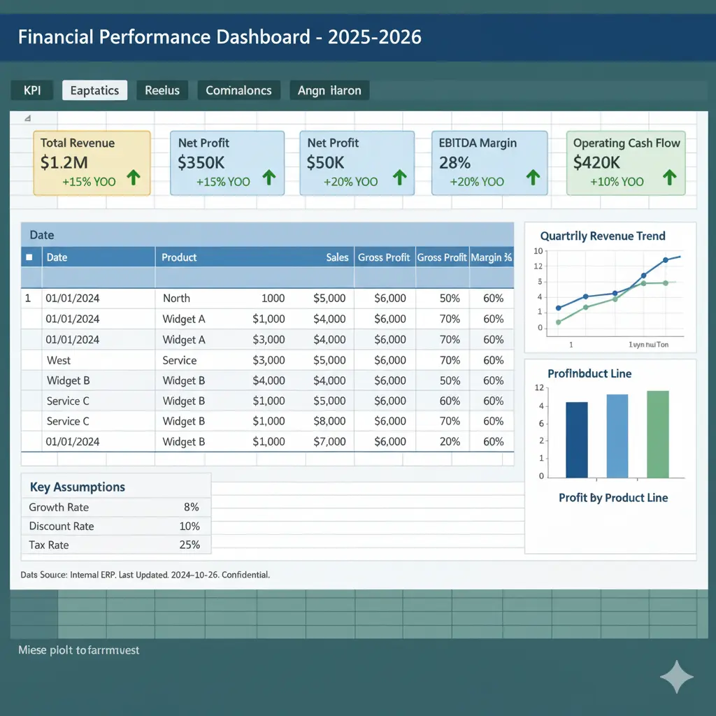
A dashboard is the final, polished product of your analysis—a visual interface that communicates the most important KPIs at a glance.
6.1. Visualizing Financial Analysis with Excel Dashboards
- Choose the Right Chart:
- Trend Over Time: Line Chart.
- Category Comparison: Bar/Column Chart.
- Part-to-Whole: Stacked Bar Chart or Waterfall Chart (for bridge analysis).
- Performance vs. Target: Bullet Graph or Gauge (use sparingly).
- Variance: Conditional Formatting with Data Bars.
- Keep it Simple: Avoid 3D effects and cluttered backgrounds. Use a consistent, professional color palette.
- Highlight Key Information: Use a single, contrasting color to draw attention to critical metrics or significant variances.
6.2. Interactive Controls with Form Controls & Slicers
Link your charts to Slicers and Form Controls (like drop-down lists or option buttons) to allow users to filter the entire dashboard by Region, Product, or Year. This transforms a static report into an interactive analytical tool.
6.3. Dynamic KPI Cards
Use simple formulas linked to your data model or PivotTables to create headline KPI cards.
excel
=LET(
    CurrentSales, SUMIFS(Sales, Date, ">="&EOMONTH(TODAY(),-1)+1, Date, "<="&EOMONTH(TODAY(),0)),
    PriorSales, SUMIFS(Sales, Date, ">="&EOMONTH(TODAY(),-2)+1, Date, "<="&EOMONTH(TODAY(),-1)),
    Growth, (CurrentSales - PriorSales)/PriorSales,
    "Revenue: " & TEXT(CurrentSales, "$#,##0") & " (" & TEXT(Growth, "+0.0%; -0.0%") & ")"
)
This formula creates a dynamic text string showing current month sales and the growth rate vs. the prior month.
Frequently Asked Questions (FAQ)
What is financial analysis in Excel?
Financial analysis in Excel involves using the software’s tools—like formulas, PivotTables, and charts—to evaluate financial data, assess business performance, forecast future results, and support strategic decision-making. It’s the process of turning raw numbers into actionable insights.
What are the most useful Excel functions for finance?
The most useful functions include SUMIFS for conditional sums, XLOOKUP for data retrieval, NPV/IRR for investment appraisal, PMT for loan calculations, and the dynamic array functions like FILTER and UNIQUE. A solid grasp of IFS and LET also significantly improves model efficiency and readability.
How can I create a financial model in Excel?
Start by creating a separate ‘Assumptions’ sheet for all inputs. Then, build your three core statements: the Income Statement, Balance Sheet, and Cash Flow Statement, ensuring they are dynamically linked. The Balance Sheet must balance, serving as a key check. Finally, incorporate scenario analysis using Data Tables and build a summary dashboard. You can learn more about Excel’s specific financial functions on the official Microsoft Learn website.
Is Excel better than Power BI for financial analysis?
It’s not about one being better, but about using the right tool for the job. Excel is superior for deep, cell-level calculations, building complex, bespoke financial models, and ad-hoc analysis. Power BI is better for connecting to very large datasets, creating enterprise-level, interactive dashboards that refresh automatically, and sharing reports across an organization easily. They are often used together in a professional workflow.
Conclusion: From Data Cruncher to Strategic Advisor
Mastering Financial Analysis in Excel is a journey that blends technical skill with strategic thinking. It’s about more than just formulas; it’s about building a logical, auditable, and flexible framework for understanding business performance and predicting future outcomes. By applying the principles, functions, and techniques outlined in this guide—from the foundational SUMIFS to the advanced Power Pivot data model—you equip yourself to not just report on the past, but to illuminate the path forward.
Your goal is to become an architect of financial insight, using Excel as your primary tool to build clarity from complexity and drive informed, impactful business decisions.
Download our free Excel template: ‘The Startup Six: A Foundational Financial Model.’ Simplify your startup’s financial planning instantly :